Do Path Signatures Generalize?

1. Why this test

Commodity prices are a hard forecasting problem. They are non-stationary, they jump regime, and a large share of the move is close to a random walk. Classical indicators can describe a window that has already happened. They are expensive to maintain, and they overfit the regime they were tuned on.

Path signatures come from rough path theory. A signature is a stack of iterated integrals along a path. Low-order terms record the net move. Higher-order terms record how the coordinates moved together, and in which order. The same shape gives the same signature if it is travelled at a different speed, and a truncated signature is already enough, because the higher-order terms shrink quickly. For a trading model that is a geometric summary of the recent path, with little hand-built feature work.

Signatures are already used in finance for pricing path-dependent payoffs, for execution, for clustering, and inside deep or kernel models. Those studies usually wrap the signature in a larger construction, or they score it on synthetic paths. What was missing was a plain test. Take the raw signature of a real commodity path, give it to an ordinary classifier, and see whether the trades still work in a later regime, on more than one asset, after costs.

This study does that. It compares signature features with a large set of ordinary open-high-low-close-volume features under the same labels, the same walk-forward, and the same costs. The useful output is a map of which design choices survive the change of regime, and a record of how far the resulting books actually go.

2. Data and empirical setup

Markets and split

The series are continuous front-month futures for WTI, gold, silver, and natural gas, aggregated from minute bars to hourly bars. The history runs from 2010 through 2023, about 15 years. Decisions use 2014–2022. The years through 2018 choose the design, and 2018 is kept out of the fit as a holdout. Parameters are then frozen and scored once on 2019–2022, a window that includes the COVID shock and the volatility that followed. Nothing in the fit is allowed to look at that window.

Labels and weights

The target is López de Prado’s triple barrier. For each hourly bar there is an upper price barrier, a lower price barrier, and a time limit. The price barriers widen when recent volatility is high and tighten when it is calm, so a quiet drift is not labelled as a trend and a volatile bar is not labelled as noise. The label is +1 if the upper barrier is hit first, −1 if the lower barrier is hit first, and 0 if time runs out.

Each label looks ahead over a horizon, so neighbouring labels overlap and the sample is not independent. Training uses average-uniqueness weights: an observation that overlaps many others counts for less. At the edge of every validation fold, any label whose horizon reaches into the next fold is dropped. A fold cannot train on its own future.

Two feature sets, one backtest

The signature pipeline follows the generalised signature method. Four choices define a candidate. The path is the close, the return, or the close together with volume. The path may be augmented with time, a lead–lag copy, or a basepoint. The transform is the signature or the log-signature, at a finite depth. The window is a single lookback, or several windows concatenated. Terms are rescaled so that depth does not bury the higher-order integrals under a factorial.

The benchmark is built from the same hourly bars. It starts from 250+ engineered features: momentum, volatility, trend, oscillators, rolling moments, and volume. Fractional differentiation keeps as much memory as possible while pushing each series to stationarity. The differentiation order is fit only on data strictly before the period it is applied to. A univariate ranking then keeps the features most associated with the label. The same walk-forward, the same costs, and the same position rules are applied to both sets, so a gap between them is a gap between representations.

Models and the book

Every candidate is scored with logistic regression and with random forests. The walk-forward uses sequential, non-overlapping test folds. Training-window length and retraining frequency are part of the search, including the case of an expanding window.

Predictions become a position. Size scales with the model’s probability and with recent volatility, so the book takes more risk in calm markets and less when the market is violent. Exits follow the same barrier idea as the labels. A trade pays its cost. The three strategies that were kept were checked after transaction costs and slippage.

Performance is read on three numbers: the annualized Sharpe, the win rate, and the drawdown. Sharpe is the ranking metric. Stability across folds matters as well, because a high average that only exists in one year is a regime, not a signal.

3. How the search was run

The parameter space is large. Path type, augmentation, depth, transform, window, model class, training length, and retraining frequency multiply into 7,000+ configurations. Testing all of them in one grid would confound every choice with every other choice. The search is therefore phased. Each phase locks one design decision, and only the configurations that hold up move forward.

The rule inside a phase is the same. Configurations are ranked by mean Sharpe on 2014–2018. A low dispersion of that Sharpe across folds is preferred when two candidates are close. The 2018 holdout is then used as a robustness check: the ratio of the holdout Sharpe to the in-sample Sharpe. A large in-sample lead has to be real before it beats a more stable alternative. False-discovery-corrected comparisons, checked with a bootstrap of the mean difference, decide whether two groups actually differ.

Phase 1A compares the path itself: close against returns, then the augmentations (none, time, lead–lag, both, and a basepoint on price levels), then signature against log-signature, at depths 2 to 6 and a small set of fixed windows. Models are logistic regression and random forests, on a rolling three-year train with yearly retraining.

Phase 1B adds volume. The surviving path is extended with raw volume or with cumulative volume. Depth is capped where the feature count would explode, in particular once time and lead–lag are both on.

Phase 1C asks whether several windows beat one. Extra windows are built by concatenating lookbacks and by lagging a signature. A combination goes to the backtest only when a principal-component check says it adds rank, and mutual information says it is not a copy of features already in hand.

Phase 1D puts the engineered feature set next to the signature candidates that survived. Retraining moves to a quarterly grid, training windows vary around three years, and the model grid is widened. The top of that list is stress-tested on costs, on the labelling, and on the risk rules.

Phase 2 is the only number that counts. All choices stay frozen. The book is run on 2019–2022 with transaction costs applied. If a configuration that looked strong through 2018 breaks here, the break is reported. It is not refit.

4. Results

Close against returns

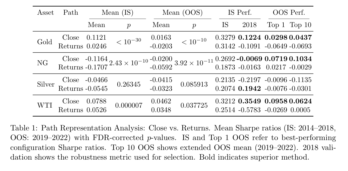
The first design choice is what the path is made of. A close path keeps the level and the cumulative shape. A return path is stationary and throws the level away.

Close paths beat return paths in WTI, gold, and natural gas, in the fitting window and on the later test. The gap is large enough that it is not a tie. Silver is the indifferent case: the two paths finish close to each other out of sample, and both drop from the fitting window to 2019–2022. The default that travels is the close.

Volume

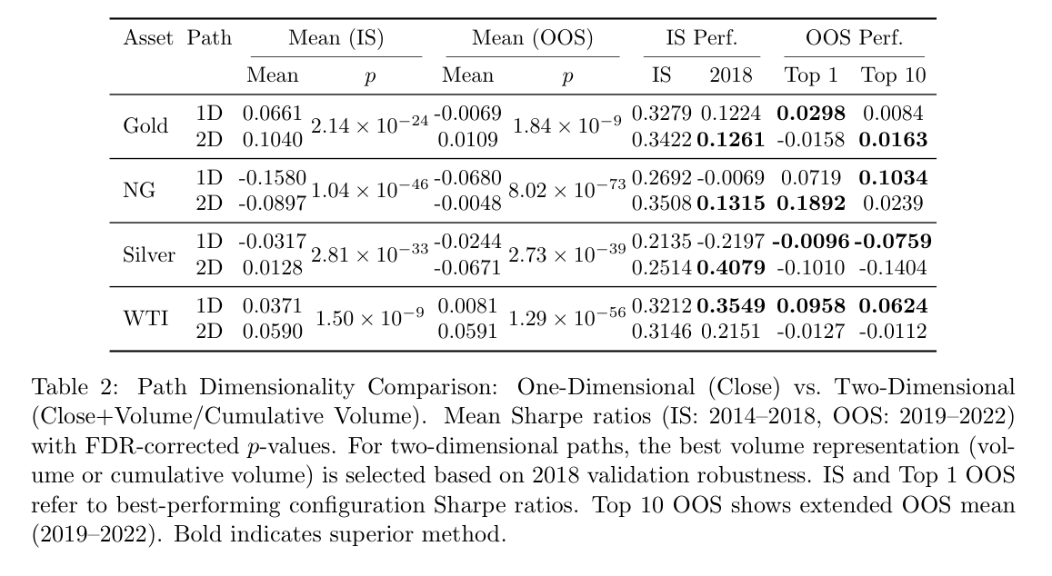
Adding volume is not a free improvement. A two-dimensional path of close and volume helps natural gas across the metrics that the selection rule trusts, and cumulative volume is the coordinate that holds up there. WTI’s best books stay on the close alone: the two-dimensional paths can look better on an average and still lose on the top configuration and on the 2018 holdout. Silver is a warning. A volume path can look unusually strong in 2018 and then fall through the one-dimensional path on 2019–2022. Gold is a tie. The practical rule is to test both and keep the one the holdout supports. There is no universal second coordinate.

Augmentation

Time is the augmentation that keeps its rank out of sample. A basepoint, added so that a price-level path is not treated as translation-invariant, does not earn a place in the default. Lead–lag sometimes scores better on 2019–2022. A principal-component check says why that gain is hard to trust: concatenating lead–lag with time adds only a few extra ranks, while the raw feature count roughly triples. Lead–lag is mostly a rewrite of the time augmentation, so a lead–lag win on the later window looks specific to that regime.

For one-dimensional paths, time, or time with lead–lag, is the robust default, and the basepoint stays off. For two-dimensional paths the choice depends on the volume coordinate. Cumulative volume already carries a cumulative clock, and the plain path or a time augmentation is then the more stable one.

Log-signature against signature

The log-signature is the compressed form, living in the free Lie algebra. On these paths it uses far fewer coordinates than the signature at the same depth, on the order of a handful to a few dozen terms against up to around a hundred.

On one-dimensional close paths there is no winner. WTI prefers the ordinary signature on the top out-of-sample book. Gold and natural gas prefer the log-signature. Silver is mixed. On two-dimensional paths the log-signature earns its place: it stays competitive, and in natural gas with cumulative volume it is the clearer of the two. Once the path grows a second coordinate, the compact transform is the one to start from.

One window against several

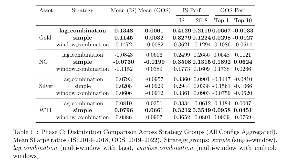
Multi-window signatures use about twice the features of a single window. They do not buy a reliable improvement.

In WTI and natural gas the single window is what the in-sample rule selects, and that selection holds on 2019–2022. In gold a lag combination is competitive. Window combinations are the awkward case: they can post a strong number in one period and fail the holdout that would have been used to select them, or the reverse. The selection rule cannot see which of those futures will be the real one. When compute is limited, stopping after the single-window phases is a sound default. The extra phase mostly spends search budget.

The frozen test, 2019–2022

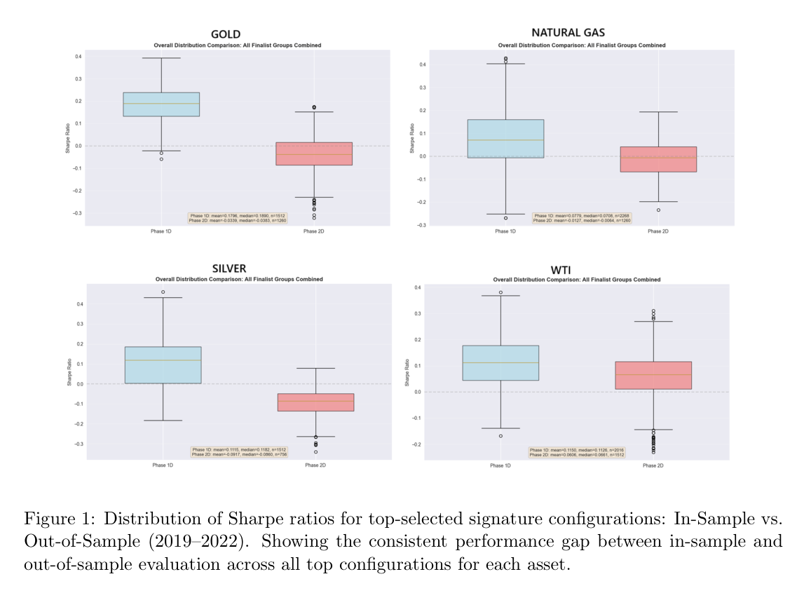
The books that survived the phases were run once on 2019–2022. Signature Sharpes on that window sit between about −0.10 and 0.18. Win rates sit near one half in every market, so the books separate on the path of returns.

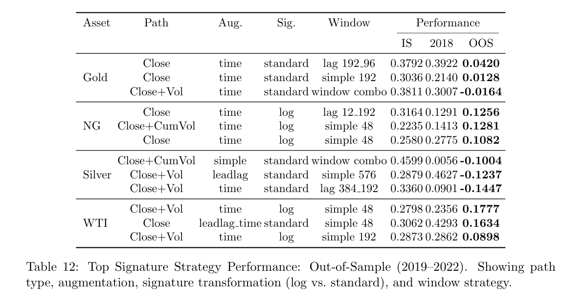
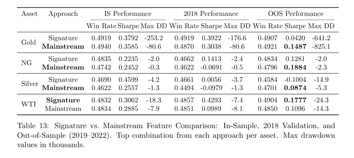
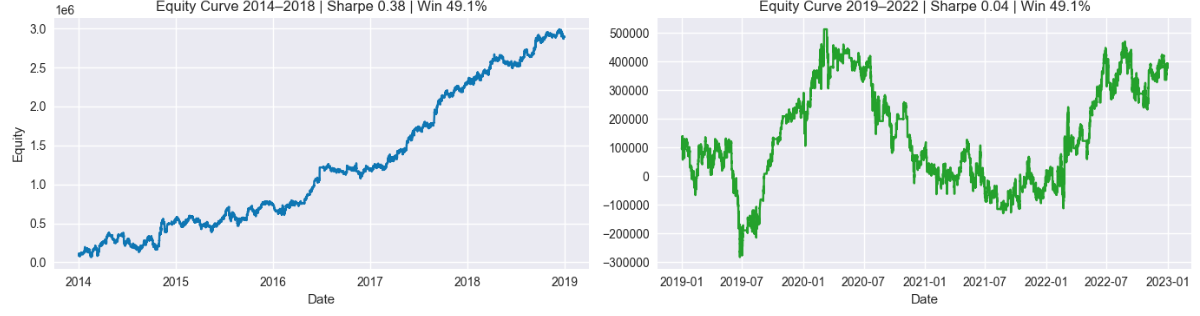
These are the leading frozen configuration of each approach, taken from the preprint tables above. In sample, the signature books led in gold (0.38 against 0.36) and in silver (0.46 against 0.26). That lead did not last. Gold kept about 11% of its in-sample Sharpe. Silver crossed below zero. The engineered books lost less ground, and in natural gas and silver they recovered after a weak 2018.

The equity curves below are Figures 2–9 of the preprint. Blue is 2014–2018. Green is 2019–2022.

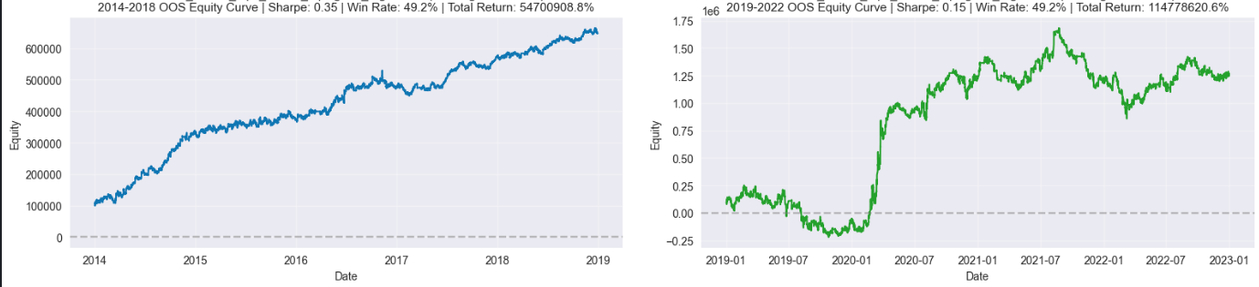
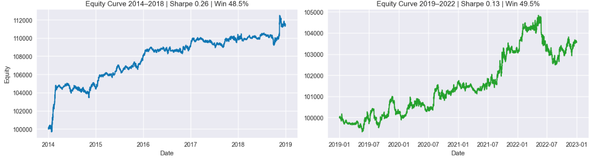
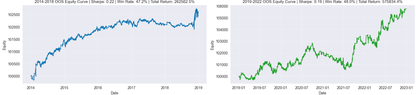
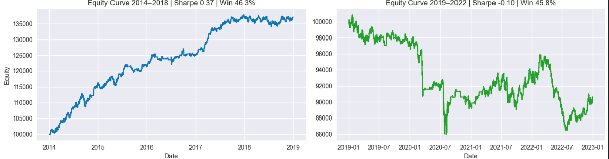
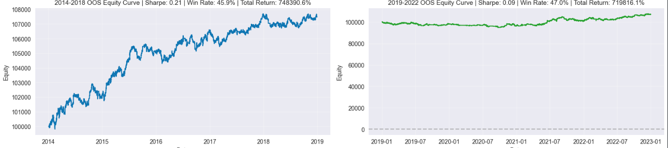
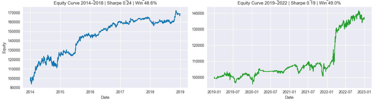
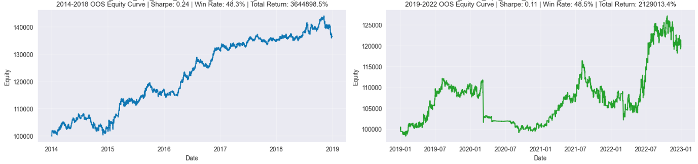
WTI is the exception. There the signature book’s Sharpe is about 0.18 against about 0.11 for the engineered features, a gain of about +0.1, and about 60% higher in relative terms. Across signature configurations themselves the Sharpes sit close together. Once the defaults above are in place, further tuning moves the result less than the change of regime does.

The whole distribution of signature Sharpes shifts down from the fitting window to 2019–2022. The selection rule kept the better part of that distribution. The level is still the level of a research book. Three of those strategies were validated out of sample with the trading team. Over the four-year window they reached about 190% cumulative net return, after transaction costs and slippage. The Sharpe improvement versus the benchmark is the WTI result above. Gold, natural gas, and silver did not produce that improvement.

5. What the map says

The phased search attributes a change in the book to one decision at a time, and it refuses a configuration that only wins inside the fitting window. The drop from 2014–2018 to 2019–2022 shows up across the distribution, so the missing profit is not one unlucky pick inside an otherwise healthy set.

Four defaults are stable enough to reuse. Start from the close. Add time, and leave the basepoint off. Use one window unless a holdout forces a second. Decide on volume per asset: cumulative volume for natural gas, the close alone for WTI and silver, either for gold. Prefer the log-signature once the path is two-dimensional.

The engineered features remain the harder baseline. They take more manual construction, and they degrade less when the regime turns. Signatures buy a shorter pipeline and, in WTI, a better risk-adjusted result. On the other three markets the engineered set finished ahead.

6. Limits

The model grid stops at logistic regression and random forests. Gradient boosting and neural nets were not in it, and a different model class could rank the same features differently. The assets are four commodity futures. Equities, rates, and currencies were not tested. The bars are hourly time bars. Volume bars or dollar bars would change the path the signature sees, because time bars bunch activity into quiet hours and busy hours alike.

The position rule can open a trade on a non-neutral prediction, so turnover carries a real share of the cost. The three retained strategies are reported after transaction costs and slippage. A richer cost model, with market impact, would move the 190% figure. So would a rule that trades only when the signal changes, or only when confidence clears a threshold.

The features are price and volume. Storage, seasonality, and supply were not added. Those are commodity-specific, and they are the obvious next coordinates if the geometric summary is going to be asked for more than it gave here.

7. Conclusion

Raw path signatures can be tested as standalone features, on real commodities, with the leakage controls a trading backtest requires. The test produces a short list of design choices that generalize, and a performance record that does not.

Close paths, time augmentation, a single window, and an asset-level decision on volume are the choices that survived four markets and a later regime. The economic result is narrower. Three out-of-sample strategies reached about 190% cumulative net return over four years, after costs and slippage, and the risk-adjusted gain versus an engineered benchmark was about +0.1 Sharpe in WTI alone. On gold, natural gas, and silver the engineered set finished ahead, and signature books gave back more of their in-sample Sharpe when the regime turned.

The part worth carrying into the next study is the map, and the phased search that produced it. Richer models, other asset classes, and other bar types can be plugged into that search. The present evidence says where a signature pipeline should start, and how much of a trading result it has actually delivered.